Sometimes formulas are not as clear as they could be. A formula that looks like '=C2*C5', for instance, is much harder to understand at a glance than one that reads, say, '=TaxRate*C5'. You can create formulas that use names (like 'TaxRate') instead of cell references (like 'C2') if you give common names to the cell or cells containing data you use repeatedly in calculations.
To name a range, click the cell or select the range of cells to name. From the Ribbon toolbar, choose Formulas, Define Name, and then type a name in the Name box. The name should start with a character, not a number, and although you can't use spaces, you can use an underscore character if you wish. Click OK.
For example, if you were to name a cell 'TaxRate', later on you could use that name in a calculation, such as in the formula '=TaxRate*C5', which multiplies the value in cell C5 by the value of the cell you've named 'TaxRate'.
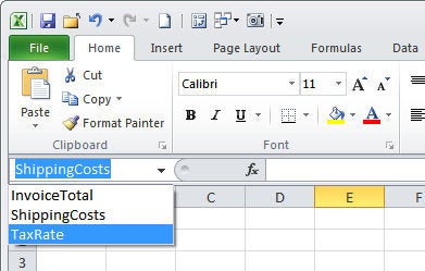
When you have named cells on a worksheet, you can find any of those cells or ranges by clicking in the Name box, which appears at the far left of the Formula Bar under the Ribbon toolbar. Click the drop-down arrow in the Name box to view a list of all named ranges, and click one to go immediately to that area on the worksheet:

Was this article helpful?
That’s Great!
Thank you for your feedback
Sorry! We couldn't be helpful
Thank you for your feedback
Feedback sent
We appreciate your effort and will try to fix the article
